In tomography problems, we are basically sending signals through a material/area, and trying to figure out that the inside is composed of. We can send signals from various places and have receivers at various places. This also gives opportunity from exploring underdetermined and overdetermined situations. In this case, we can picture a situation where we want to determine a material by the use of sound signals. The physical details include slowness s(x), which is the inverse of velocity, which is determined by the material. If the ray goes straight, it will continue to go straight and not bend at interfaces, which simplifies the forward problem.
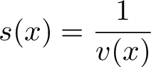
The forward problem, the time it takes for a signal to travel, will be the slowness multiplied with the distance travelled
The advantage of using slowness compared to 1/velocity(x) is making the forward problem linear, and, putting model parameters to 0, i.e, 0 slowness means the signal travels instantly, compared to setting velocity(x) as infinity. This is seen in e.g the spike test below, where we can set slowness to 0.
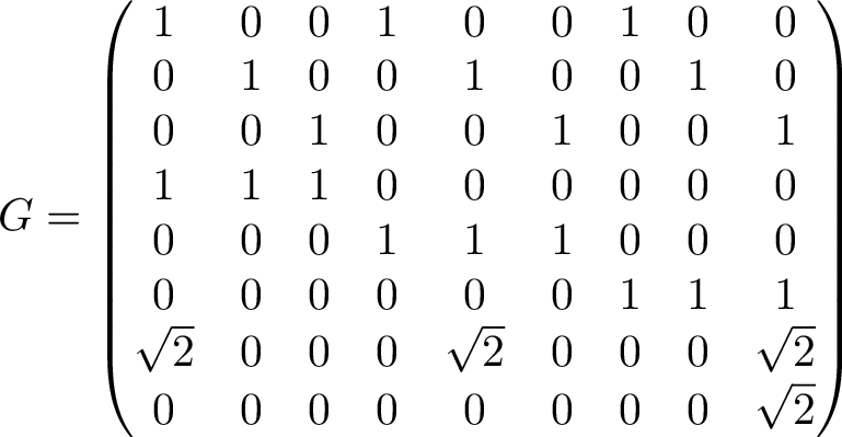
The design matrix is given below. We have 8 rows, for 8 measurements. We have 9 columns, because the measurement area is divided into 9 blocks of assumed constant slowness
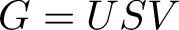
U is for data space V is for model space S contains singular values One can also get singular values by calculating eigenvalues of G^TG or GG^T. The SVD can also be used for find a generalized inverse of G. Imagine we can't get G^(-1) directly, but we CAN get G = USV^T G^TG does not always exist. A solution for the underdetermined case is m = G^T(GG^T)^(-1)d but, for numerical accuracy issues, it is better in practice to use SVD. Same thing for overdetermined least squares, it's better to use SVD. We basically these cases: 1) m=n=p 2)m = p and p < n 3)n = p and p < m 4)p < m and p < n We can have a sitation, where infinite models m can give the same data d. And we can have a situation, where infinite data d, can give the same model m.
Using SVD to solve the inverse problem
Example from chapter 7 from Tarantola book
We have 9 parameter slowness model, but we only have 8 travel time observations. The singular values are
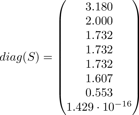
Worth noting here, the last singular value is 0, ignoring numerical error. The ratio of the largest singular value to the smallest remaining singular value is thus about 6 = 3.180/0.553 The generalized inverse will thus be stable in the presence of noise. Rank(G) = 7 = p, and we have n = 9 parameters, and m = 8 observations. Thus, p < m < n. The problem is both rank deficient, and will in general have no exact solution.
Spike test
In the spike test, we set a block with a value e.g 1, and the rest 0. Thus we are saying, that the signal travels through some blocks infinitely fast, and 1 other block it will go through slowly.
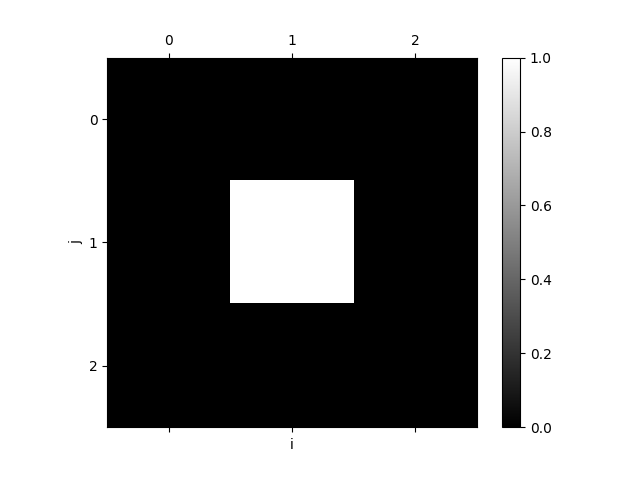
Spike test, middle block i.e 5th element is 1 and rest 0
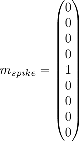
Spike test model parameters
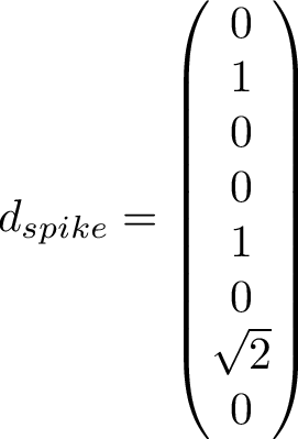
The spike test leads to the following data, assuming no errors
The SVD solution based on spike test
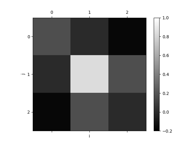
Spike test, solution plotted
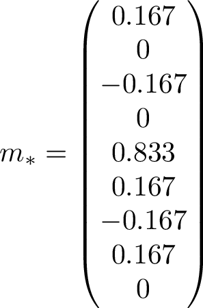
Spike test model parameters solution inverse
Eventhough the errors are zero, we do not get a perfect solution. However, we see that in general the inverse solution captures the true model parameters very to some extent, and especially the fifth element is larger compared to the rest. We DO howevever get a solution that is equal to the test data.
We can get the resolution/variance of a parameter. Similar to ANOVA, with beta/sigma for parameters. Certain parameters of the model can be estimated more clearly than others, maybe they have more measurements going through them, or lower measurement error.
Model null space
We can see nullspace. m9 is uniquely determined by obs 8, so it isn't in the nullspace, i.e i can't add to parameter 9 and still obtain same output from G(m+km0) = d, this only works when m0 is 0 for 9th block. The 9th and 8th column of V gives the nullspace,
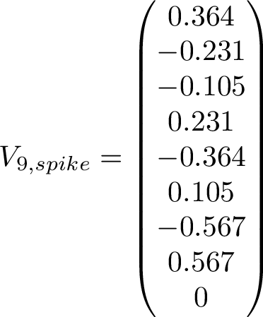
Column 9 of V matrix
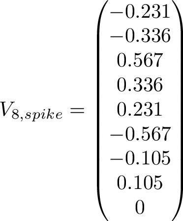
Column 8 of V matrix
Any linear combination of a model m, and V9 and V8, will result in data that comes from just model m alone, as shown below:

This shows that infinite models can fit the data, and the model m we get from SVD is just the one with least norm. Whether that one particular m is physically realistic, should also be investigated, and if not, perhaps correcting it with the nullspace to better match physical material values.
Data null space
The U matrix is associated with the data, and the last column in this case, is the null space vector. We can add this vector with a constant to the observed data, and we will still get the same model from inversion! The null space vector is the 8th column of the U matrix:
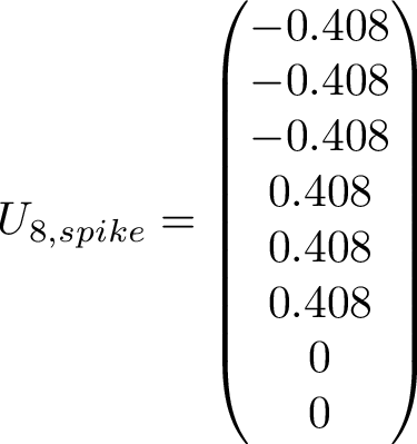
We see that the last 2 entries are 0, which means, we cannot add anything to the last 2 observations, without changing the resulting found model. This is geometrically obvious for the 8th observation, which goes through only the 9th model parameter diagonally (9th material block). Adding U8 to the data vector, will result in the same model m* as found before:

Here U8 is only the 8th column of U, being the column vector. Whereas Up, is the matrix by taking all columns of U up to column p = 7.