2D Ising model

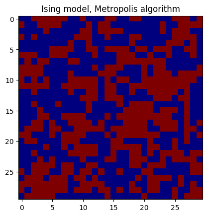
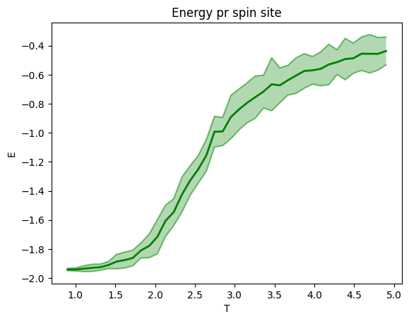
This model simulates ferromagnetism. Neighboring electrons affect each other through magnetic fields generated by their spins. The overall potential energy is reduced when neighboring electron spin point in the same direction.The 2D Ising model sets up a square lattice with each site representing an electron spin with direction up +1 or down -1. Ferromagnetic behavior shows when there's a majority of spin either up or down, which can happen at a low temperature. At high temperature the thermal disturbances will randomize the direction of the magnetic dipoles(electron spin) such that the magnet becomes a paramagnet, losing its ferromagnetic properties. Multiprocessing has been used for the parallel processes, giving significant speedup.

The Hamiltonian of the system is given by

We see here the spin lattice at T = 2.45, slightly higher than the critical temperature. Domains are still visible, with red being spin up, blue being spin down.Started from random configuration.For T = 4.85, the thermal disturbances are too strong for any significant domains to develop.

Various statistics and physical quantities can be computed from the Ising model. Error bars are added assuming normally distributed statistics, with 95% confidence interval, corresponding to +-1.96std/sqrtN. This is somewhat crude, and occasionally unphysical, but gives a good idea of the thermal variations. Alternatively we can look at the median, which may be more robust. 95% confidence intervals come from bootstrapping, which means essentially drawing(with repetition) from the empirical CDF

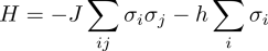
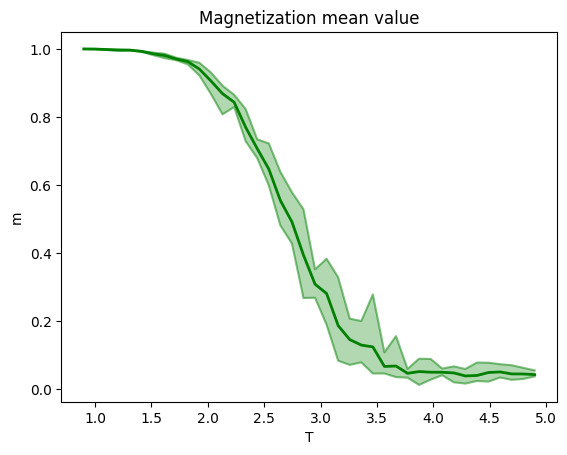
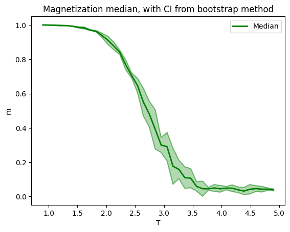
The magnetization is a measure of alignment and order, and therefore strength of the magnetic field from the magnet. Magnetization can be negative or positive depending on which way the macroscopic field is oriented.Magnization is higher at low T, if you start from an ordered state, than at high T, since the thermal disturbances will break alignment.

The magnetization pr. site is given by

Energy pr spin site. At low T, starting from an ordered state, the dipoles will try to be put into the lower energy states, as specified by the energy from their neighbors.

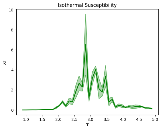
The susceptibility is a measure for how the material reacts to an external magnetic field. If x_v is positive, the material is more paramagnetic, and the dipoles inside can align to a greater degreewith the external field. The models gives low susceptibility for low T, since the dipoles are firm in their arrangement. Higher T will make the dipoles more free to be influenced by an external field, but,too high T means the thermal disturbances will be too strong to give any significant alignment with an external field.

The magnetic susceptibility can be found from the variance of the magnetization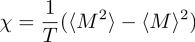

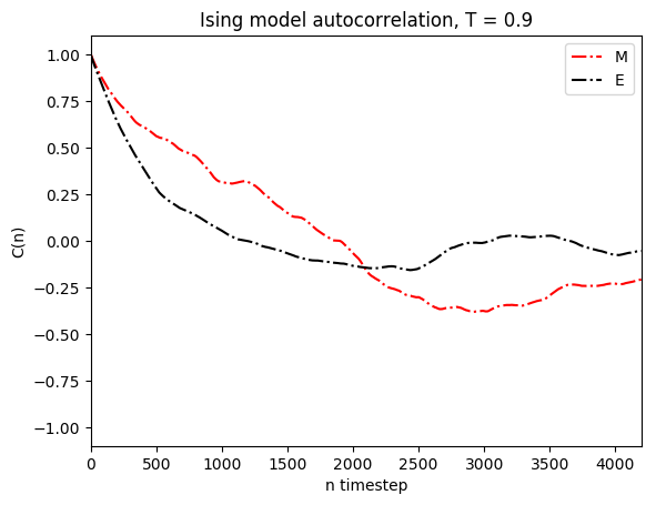
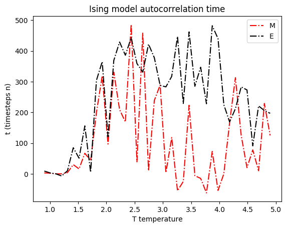
The result is seen below

The specific heat describes how much the internal energy changes when the temperature changes. We see that the internal energy changes mostly around the critical temperature, which can also be seen from the energy graph.Once the magnetization reaches 0, and the energy reaches it's maximum, we basically have random configuration of spins, and increasing T cannot do anything to increase the Energy in this system.

Specific heat from the simulation is seen below

Autocorrelation

To have meaningful average values we need independent and uncorrelated data. Since we change the spin states one site at a time, consecutive states are highly correlated and thus any statistics aswell. Looking at the autocorrelation times we get a sense of how many steps should be between each measurement.Two statistics can have different correlation times, so the safer practice is to pick the longest correlation time. For large t values we're calculating a large lag. This also means that the larger lag autocorrelation we calculate, the more error-prone it is, since we'll have fewer points to calculate the autocorrelation from. Hence, first we will see autocorrelation drop off approximately exponentially, but then the lack of measurements will start to create noise in the autocorrelation function, making wild oscillations and peaks etc. So here we cut off the autocorrelation plot at 0.7*tmax, so the noisy tail isn't visible.Integrating the autocorrelation values gives the integrated autocorrelation time. In a sense it's a more direct way to get the parameter for exponential decay compared to fitting and doing least squares etc. The integrated autocorrelation time calculated is then used in collecting data to avoid correlated data.

We can see integrated autocorrelation time for different temperatures. Near the critical temperature we have large clusters, so the spins are not likely to flip. Also, the temperature is low enough that the probability of flipping based on thermal disturbances is not that high either. So we have higher correlation time at Tc. When the temperature increases further, we begin to break up clusters and also increase the chance of flipping spins due to thermal disturbances, so the autocorrelation time decreases.

Link to project on Github

2D Ising