Seismometers can behave like pendulums and have oscillations, which complicates the picture when trying to see what oscillations come from actual seismic activity, and which oscillations are just due to the instrument itself. For a series of disturbance inputs, the instrument itself will be very visible in the data. We can look at an ideal case, where the pendulum is critically damped, such that after an initial disturbance, the seismometer will settle down to rest, without any oscillation. We can then ask, given the instrument impulse response, and a graph, what were the seismic inputs? This gives rise to an interesting case of inverse problems that are also ill-posed.
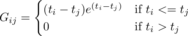
Suppose that the seismograph is critically damped, such that the impulse response decays, without oscillations, from an initial impulse. One such impulse response could be given by the equation,
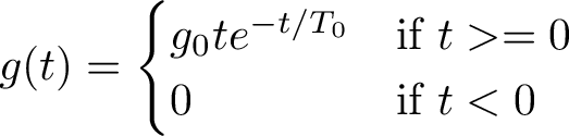
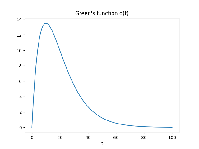
Where T_0 = 10 and g_0 = T_0*exp(-1). The instrument impulse response (scaled to max response = 1) is plotted below
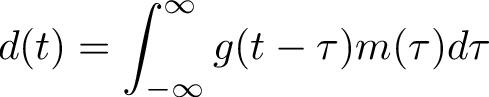
The true data i.e measurement of the seismograph can be expressed as the general convolution between the Green's function and the true model
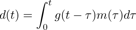
The true model is 0 for t<0, so we can change the lower limit to 0. The impulse response is also 0 for t<0, and thus when we reflect it on the axis in the integral, it will only have values up to t. So we can also change the upper limit of the integral. This helps with discretization, as we of course rather want to avoid discretizing the entire axis from negative infinity to infinity.
The integral can be discretized and expressed as the linear model
Where the discretized G matrix is given below. The final G matrix will be further rescaled with 1/max(G)
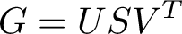
We will solve the inverse problem using singular value decomposition on the matrix G,
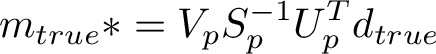
The solution can then be expressed as below. Note, except for the trivial S inverse,there are no inverse matrix! Assuming the method and algorithms behind it are stable, this is a huge advantage compared to solving the normal equations directly.
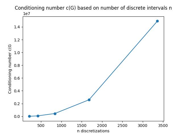
The conditioning number is cond(G) =70000 is ill-posed. It is also moderately ill-posed? because the singular values don't cut off quickly to 0, but rather descends slowly towards 0. There is no clear cutoff where can we say the singular values have reached 0.
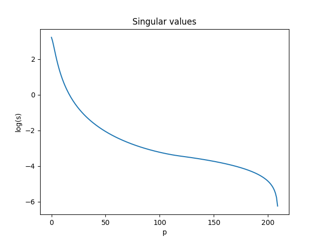
The conditioning number increases as we make more discrete intervals to approximate the integral. This suggests that also choosing the right discretization can have an influence on results, depending on method.
Test model
We will use a true model being the sum of two gaussian peaks, with the width sigma = 2

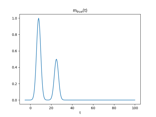
Our goal is to reconstruct this model, using the method described above. Note again here, that we are actually not trying to find the six parameters. We could probably ALSO do that after, by setting it up as another inversion problem. The strength here, is that we do not have to set up a particar model function or type or class. We will simply let the instrument impulse response, along with the discretized integral as Gm, find all the peaks presents in the signal.
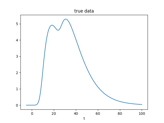
Data - with and without noise
Solving the convolution from t = -5 to t = 100 gives the true data below
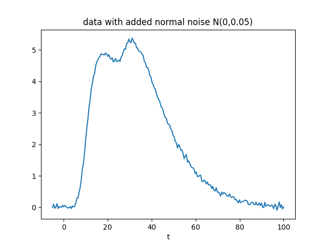
If we add some noise to the solution we end up with following observations
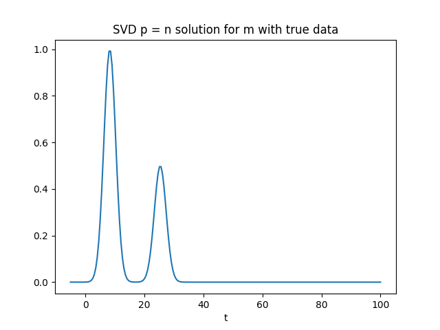
1) Solution with all singular values (p = n)
Keeping all singular values, we see that we are able to reconstruct entirely the real signal. However, adding a small amount of noise to the signal, the reconstruction fails catastrophically.
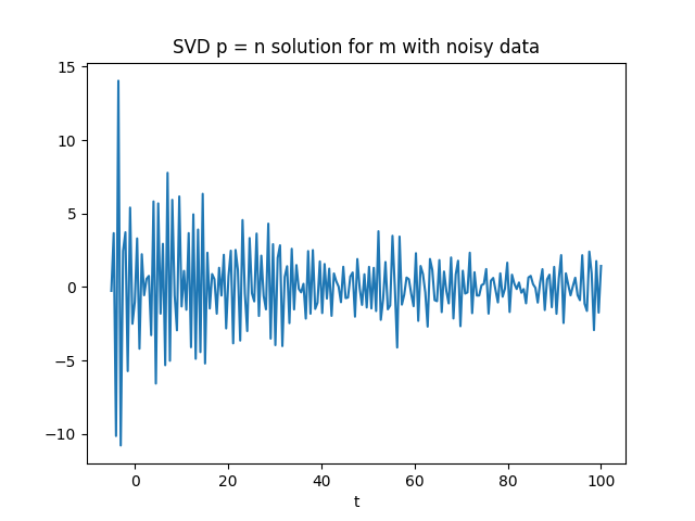
We see here that using all singular values, we do have have what looks like 2 disturbances. However, these disturbances also reach very large negative values, while the true model is always above zero. So the solution is highly unstable and has a lot of variance.
2) Solution with truncated SVD (p = 26)
A good solution is p = 26. We see that we reduce the variance A LOT for the noisy data.
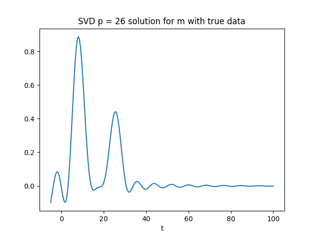
We see that the SVD solution no longer captures the true model m(t) when using just 26 singular values. We also see some bias/shrinkage, in that the peaks don't reach the same height as the true model. The peaks also appear sligtly wider, so we lose some resolution.
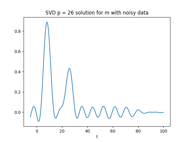
We see here that we actually capture our true model reasonably well! Also compared to using full p = n, our solution is much more stable, and only modestly goes below 0 on the y-axis.
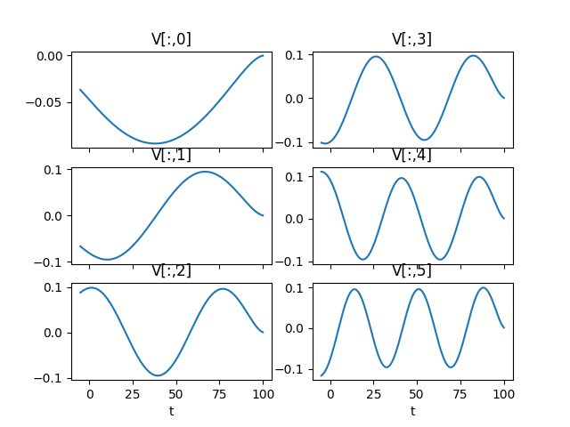
Why oscillations? - columns vectors of V
We see that for p = 26, there are oscillations in the solutions. The oscillations come from the column vectors of matrix V. The first 6 (corresponding to p = 1 to p = 6) column vectors are shown below. We see that as p increases, each vector has more zero-crossings and is a higher frequency oscillations. If we want to capture very sharp peaks in our solutions, we have to use a high p value - otherwise the peak can be smeare out greatly.
References
Richard C. Aster, Brian Borchers, Clifford H. Thurber - Parameter Estimation and Inverse Problem (2ed)