Finding earthquake hypocenters. We solve it here using Gauss-Newton and Levenberg-Marquardt methods, which are methods for nonlinear optimization, specifically with nonlinear least squares in mind. The inverse problem is nonlinear, even for the ideal case of isotropic medium giving constant velocity profile. Velocity depends on density, elasticity and wave type of the medium, and largely tends to increase with depth for roughly the first 2000km, going through the crust and mantle. Different wave types include body waves and surface waves, with surface waves usually causing more damage. due to larger particle motion/displacement. Due to the large velocities, seismic waves can travel many kilometers pr second, accurate travel times are important in order to compute a precise hypocenter. Being off on travel time by even half a second, can mean that the estimated hypocenter can be off by many kilometers.

The total travel time is basically the sum of the travel time in each layer t = d/v for distance d and speed v, here written for a two-layer model. tau is an initial time offset, which becomes especially important if multiple earthquakes happen almost simultaneously.
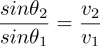
Counting angles from the normals to the layer interface separating areas of velocity v1 on one side and v2 on the other side, Snell's law is
To solve the nonlinear least squares estimate, one often used method is the Levenberg-Marquardt algorithm, which is essentially iteration of the following system of equations

Along with the model update
where the gradient is given by

for functions fi that are the weighted residual of each datapoint, giving Nobs functions in total
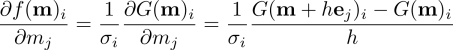
Bold f is the vector containing all Nobs residual functions. Calculating the gradient doesn't seem feasible, even for simple setups using Snell's law. Finding the intersection point is done with an iterative solver, thus finding the deritative is a problem. In this case finite difference is often used. Since the forward problem depends on G(m),
The Hessian is given by
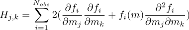
Which is approximated, assuming the first term is much larger in magnitude than the second term

The cases where convergence can be expected is, first, when the function values f_i(m) are small in magnitude, at least near a minimum. Second, if the function is only mildly nonlinear, then the second derivative can be assumed relatively small.
Two-layer model Earthquake hypocenter location
A subproblem is finding the x_(i,j) horizontal interface position for the jth sensor station. From Snell's law and some trigonometry we can arrive at the following nonlinear equation

With two layers, one roughly representing the crustal zone with v = 5km/s and beneath it the mantle with v = 8km/s, assume an earthquake happens at (40km,-70km,0.5s), and an initial guess relatively many km off. Most events occur shallower than about -40km depth, so -70km is pretty typical.
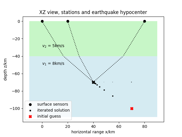
Above is seen the physical situation, with three sensors on the surface. At the layer interface kinks in the ray path can be seen, as the waves that travel from the earthquake to each sensor, will be the ones that go there in least time, as according to the very general least action principle which often appears in physics. It can be seen that the method converges to the solution very reliably. Total steps of the LM algorithm is around 400, and only every 50th iterative model is shown. The iterated solution is very close to the true solution. In real life situations, location of earthquakes around the world are accurate to within 10-50km.
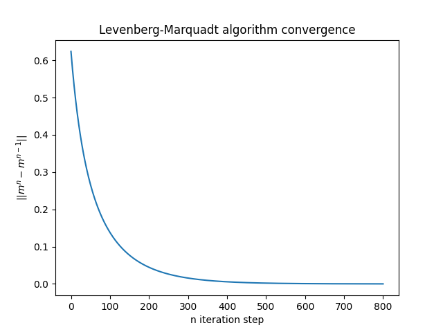
For the norm of succesive models, it can be seen that convergence happens after a couple of hundred iterations, and the algorithms stops near 800 iterations. Using smart methods to update algorithm parameters can speed up the process.