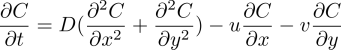
For a fluid that disperses a chemical, we can try to find out the release history. Applications for this are e.g. groundwater contamination, to find out how much chemical was released, when it was released, and where it was released. Usually we go forward in fluid dynamics, by starting from some initial conditions, and knowing the physics of the situations, we can integrate the system forward and obtain variables at a later time. There are many methods for this, the simplest are usually analytical or finite difference methods. We usually ask for the forward integration, for example in weather forecasting. The reverse question is more rarely asked, i.e, looking at a fluid system, we may want to ask how it started to eventually reach that configuration. This question can be a bit harder to answer, due to turbulence/chaos in fluid simulations, and in general, many initial configurations can lead to the same outcome. The advection-diffusion of a chemical in a fluid, e.g down a river or by pipes, denoting its concentration C(x,t), can be described by the PDE
the velocity v_a = (u,v) is assumed known and likewise the diffusion constant D = D_x = D_y. The RHS can also include sources,
With point sources we can find an analytical solution to the PDE, for a given point x and time t. Note that this is actually a pretty extensive calculation for each grid point
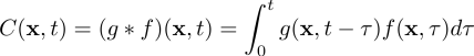
Where g(x,t) is Green's functions, which solves the equation assuming a point source(delta function). Here f(x,t) will be a source function composed of point source released at 3 points in space, with the chemical being released at different points in time at each source. The source function Csources(x,t) = f(x,t) can be written as a sum of delta functions

For the PDE we can find the following Green's function, which usually comes from writing the PDE as a linear operator L, and solving LG(x,t) = delta(x,t) for G(x,t).
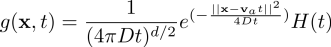
where H(t) is the Heaviside step function and d=2 is the number of physical dimensions. The release history reconstruction can be put into the formalism of an inverse problem with matrix notation, where in essence we are solving
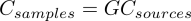
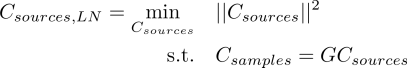
The unknown model parameters are here the concentration sources Csources(xsources, t) throughout time from t = 0 to T, where all the concentration samples Csamples are taken at time T, and G is the design matrix, made up of the transfer function of the problem, i.e the Green's function of the observations/samples.
For N samples and Nt times to be computed, and here using only one source. For multiple sources, the column dimension of the matrix increases as (Nt*Nsources) and thus also the number of parameters to be estimated. The design matrix and measurement values can then be used to find model parameters (concentrations sources) with different methods such as Least Squares, Ridge, Lasso, etc. We may also want to impose other restrictions, such as Csources(xsources,t) larger than zero, i.e exclusing solutions where the sources become sinks, if we know that pollutant was only added to the river, and none if it was cleaned up.
The forward model with the spread of pollution is animated. The inverse problem is to find how much each source has contributed to the pollution, by measuring samples at random points.
Overdetermined system
We can look at the overdetermined and the underdetermined cases and various methods of finding the model
Ridge solution - L2 norm on misfit, L2 norm on parameters
Since I don't have any data I will construct a situation and calculate the forward solution using the above equations. Data samples are then taken from the analytical solution, with Gaussian noise 40*N(0,1) added in this example.

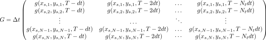
Using 3 sources, with a fluid flow changing from east to northeast, the chemical concentration is transported and diffused with time. Sampling at random places, we can try to reconstruct the concentration field.
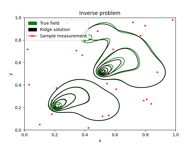
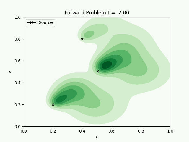
Sample points(red cross X) are generated randomly in the domain, and here 50 samples are used. The black field is the reconstructed concentration, and the green is the true field. The black field captures the main components, and due to the regularisation parameter, slightly underestimates the spread of the concentration. The 3 sources are shown below with true concentration inputs through time, and compared with the Ridge found solution. There's high variance, suggesting we can increase the regularisation parameter a bit more and try to get a better fit. Note that the inversion gives the entire release history for each source, so gives a pretty detailed picture of how long the contamination occured.
The solution it gives is very similar to the found field though, which also suggests that the solution is non-unique. The fluid flow changes through time, starting eastward and finishing northeastward, which results in a wider section of polluted area, compared to a steady flow.
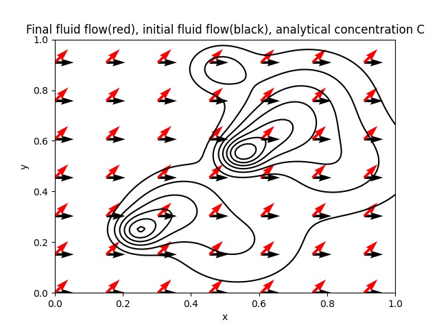
The concentration field is shown along with fluid flow vectors, red for final flow direction, black for initial. The change in direction with time could come from e.g changing winds, or rainfall falling in nearby southern hills, changing the pressure gradients.
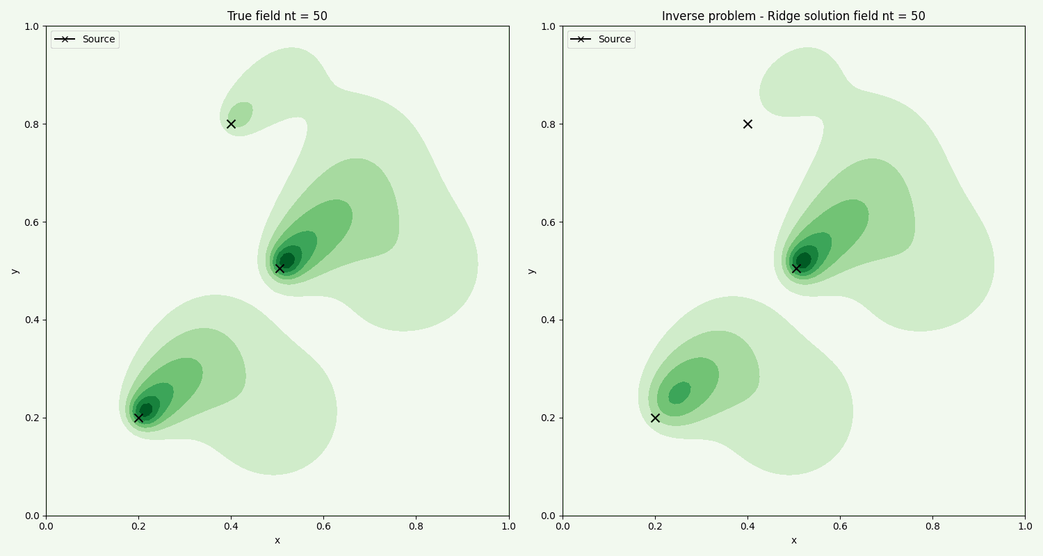
The time evolution of the actual field, compared with the field found from the inverse problem using chemical sample points. We see that the method overall captures the general flow. Further improvement can be made by fine tuning the optimization ridge parameter.
Underdetermined system
In the case of wanting to estimate the many sources or a dense time history, with only few samples/data points, we will have an underdetermined system Csamples < Csources. In this case there are infintely many solutions to the system of equations Csamples = GCsources. Instead of doing least squares then, we can do least norm solution.
The solution looks similar to the least squares solution, with switching order of operations and tranposes

For 28 data samples, trying to predict 3 sources with 10 timeframes each, we get the solution
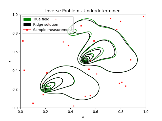
The red dots are again the random samples. The solution is not too bad and captures the overall dynamics.

Like the case for Ridge solution, the method in general captures the flow. Here we are using less samples.