An example in HMM is drawing balls from urns, where the balls have different colors, and on each turn we select which urn to draw from based on a Markov transition matrix. We assume here that the probabilities stay constant, so we should sample with replacement from the urns, and shake the urns after each draw. In the Markov assumption we assume that the next state depends only on the current state, and not any states before the current state.

Three urns with blue and red balls. AI generated.
The transition matrix, here denoted by p, is given below. The emission matrix gives us the probability to draw a colored ball from each state. Each urn may have different number of each color, so the probability to draw a red or a blue ball can be different between urns. We have 3 urns, and the matrix gives the probability to switch from one urn to another urn.
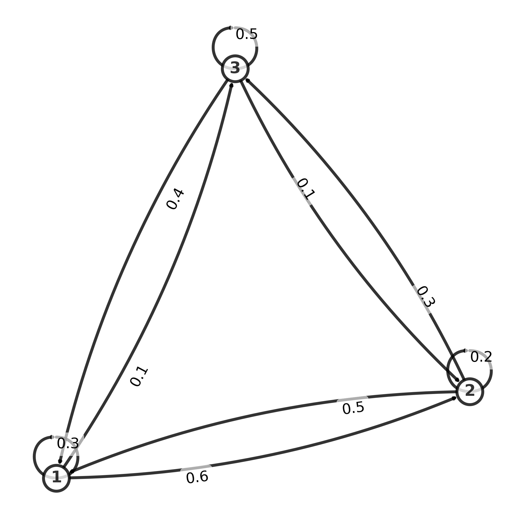
Graph of transmission matrix
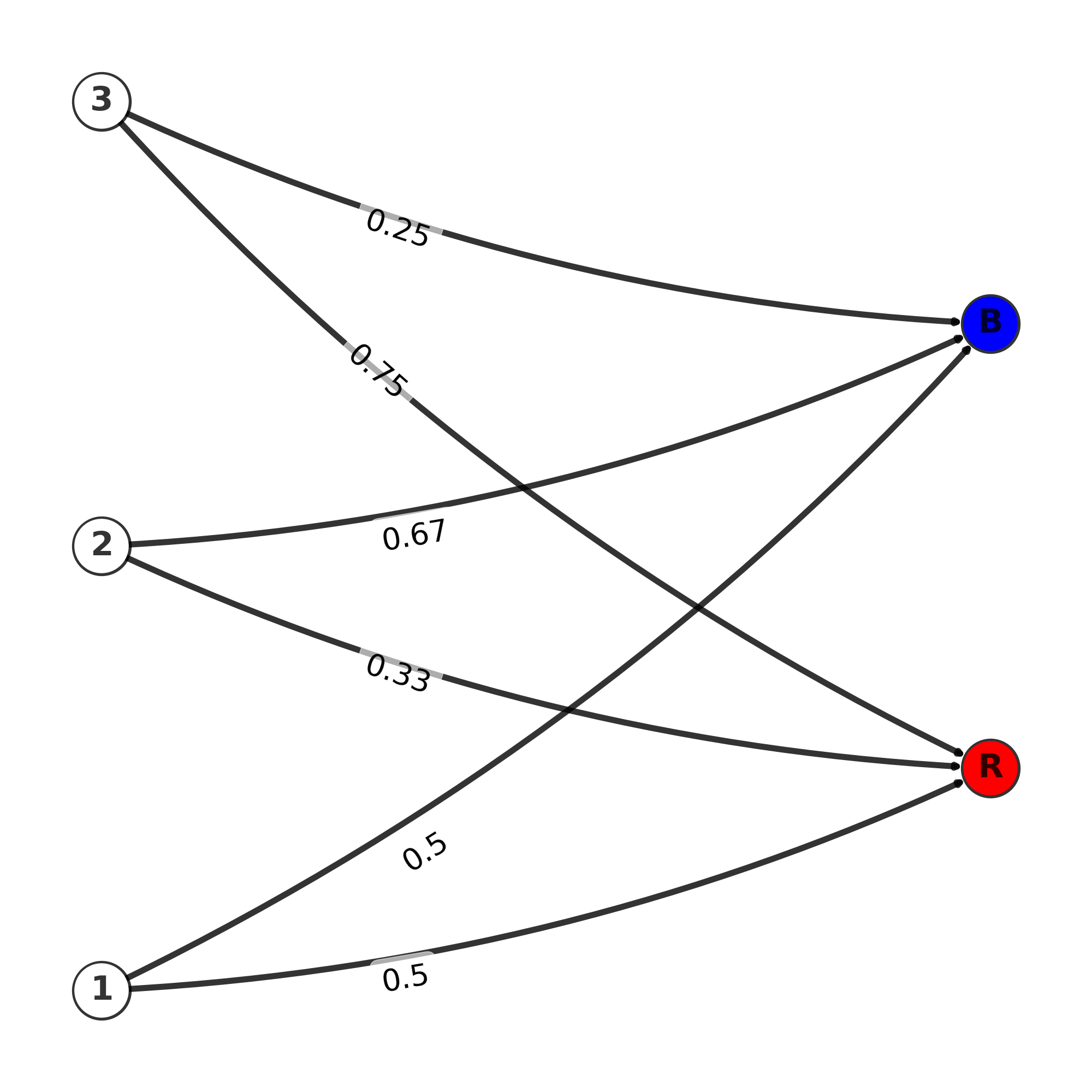
Graph of emission matrix
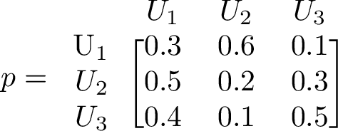
Transition matrix
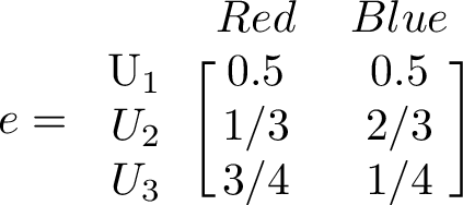
Emission matrix
The color of the ball is what we actually observe(or rather a sequence of balls), and finding out which sequence of urns they were most likely drawn from, is the problem we are trying to solve. This is one of the three fundamental problems in Hidden Markov Models. We will use the Viterbi algorithm, which is actually a dynamic programming algorithm, since it solves the problem by looking at each separately.
Steady state and eigenvectors
The Markov matrix is a stochastic matrix, so the largest eigenvalue will be 1. This means, over long time, applying the matrix p on an arbritary state vector, the result will converge to the eigenvector corresponding to the largest eigenvalue. The eigenvalues are seen below
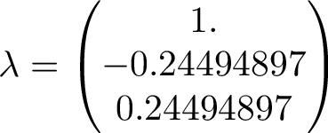
The eigenvector corresponding to the largest eigenvalue is the one to the right. We can compare this eigenvector with long term average of our simulation.
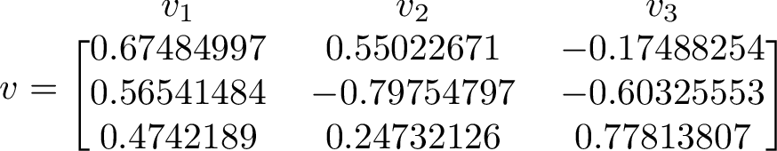
Counting how many times each state occurs and putting the counts in a vector let's us compare the right eigenvector to the long term simulated distribution. The counts from one run gave the values [0.393, 0.313, 0.294].
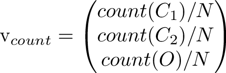
Scaling the long-term average vector to unit length and comparing it to the 1st eigenvector, we see they are indeed very close to eachother!
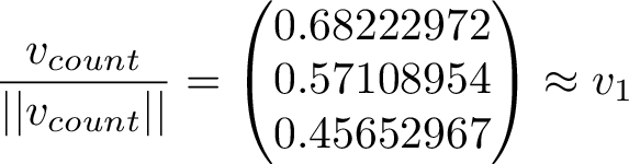
Obviously the count vector will have some random error from the simulation, and also the convergence to the 1st eigenvector is only as the simulation goes on to infinity.
Viterbi algorithm - Most likely state sequence, from a given observation sequence
If we observe a sequence of emissions, and we know the p and e matrix, we can ask the question, which sequence of states was most likely to produce that observed sequence? Note, that many paths of states could give the same observed sequence, but one path would be the most probable. There could be several paths with the same maximum probability however, in that case, the Viterbi algorithm just outputs one such path, based on terminiation rules in the algorithm. The Viterbi algorithm was implemented based on the wikipedia page, and is a relatively short algorithm. Here it is implemented as written in wikipedia, however, variants include e.g taking the logarithm of probabilities, for numerical stability, especially for long sequences.
The probability of a path comes from multiplying together the elements of the transition and emission matrix for each timestep. In the end, a path with highest probability will be singled out by the algorithm. For a sequence of observations O and a sequence of states Q, the total joint probability of that outcome is given by
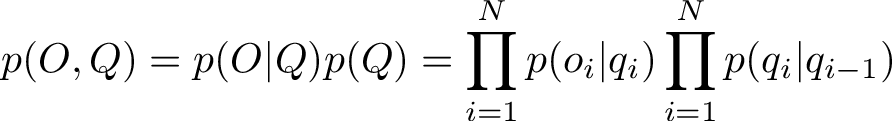
Note for the inital state i = 1 for q_1, we might select a uniform probability, in this case with 3 states we can set the initial probability as 1/3 for each. Alternatively, we could set the initial probability corresponding to the distribution in the eigenvector corresponding to the unit eigenvalue.
1) Observation test {BRBRBR}
Observing alternating blue and red balls, we can find the highest probability path with Viterbi algorithm
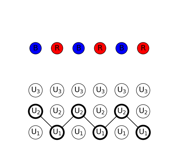
We can see that the path found is alternating between urn 1 and 2.
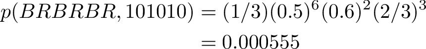
The probability of the states and observations is rather low, but it is the largest probability of other sequences that can give the same sequence of observations.
2) Observation test {RRRRRR}
A total of 6 balls have been drawn from the urns, and they are all red. We can find the path with the highest probability by using Viterbi algorithm
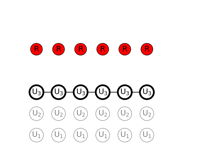
The max joint probability of sequence and observations is given below.
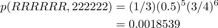
In this case the most probable path is picking only from the 3rd urn. We see that the probability to pick a red ball from urn 3 is very high, and also, the probability to pick from the 3rd urn on the next turn, after having picked from the 3rd urn, is also very high.
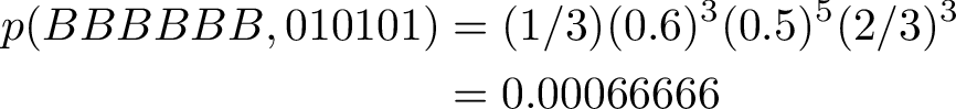
3) Observation test {BBBBBB}
We see that 6 balls have been drawn from the urns and they are all blue. We use Viterbi algorithm to find the most probable path of urns
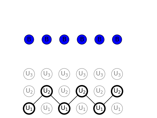
Interestingly the sequence of states is the same as for the observations set of alternating red and blue balls. The probability of only blue balls is slightly higher, so we can assume that in case we did have a sequence of alternating urn 1 and 2, it is slightly more likely to observe more blue balls than alternating red and blue.
References
https://www.cs.cornell.edu/~ginsparg/physics/INFO295/vit.pdf
https://en.wikipedia.org/wiki/Viterbi_algorithm
chrome-extension://efaidnbmnnnibpcajpcglclefindmkaj/https://web.stanford.edu/~jurafsky/slp3/A.pdf