In biology we have open/closed ion gate channels, and they can be modelled as Hidden Markov Models. Here we will rather just try to investigate how one might identify the number of states of the membrane. In general, we have one open state, for which current will flow, but we can have several closed states, for which no current flows. Those multiple states can have different dwell times. We can also assume, that frequency of measurement is higher than the characteristic dwell times of each state (Nyquist sampling theorem). We also assume, that we have observed the system long enough for all states to occur, observable and hidden states.
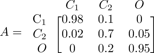
The transition matrix, here denoted by A, is given below. Each column sums to 1, since the column denotes the current state, and the rows denotes the next state, corresponding to a 100% chance. Here we have 2 closed states C1 and C2, and the 3rd state is open O. In principle here, we assume emissions for the closed states are discernable, however for ion gated channels, we really only notice two cases, which is open or closed. We will later collapse the two closed states to a single closed state, which corresponds more to a Hidden Markov Model.
Using the transition matrix we can simulate the Markov chain, by drawing random uniform numbers. An output is seen below
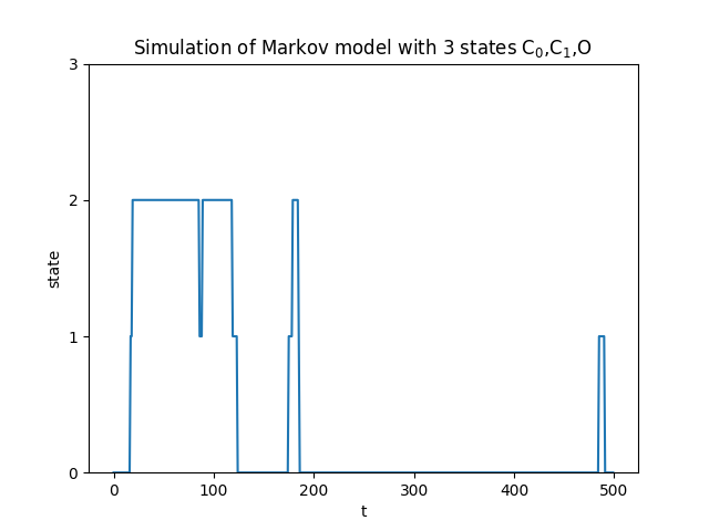
Already from a simulation plot, we might qualitatively notice that the states have different residence/dwell times, by looking for shifts in states, or how long a state remains. I.e we can see that state 0 = C_1, is a state that is rather persistent compared to state 1 and state 2. This is how however easier in a plot like this compared to a real plot, where we can only see two emission states: closed or open.
Dwell times
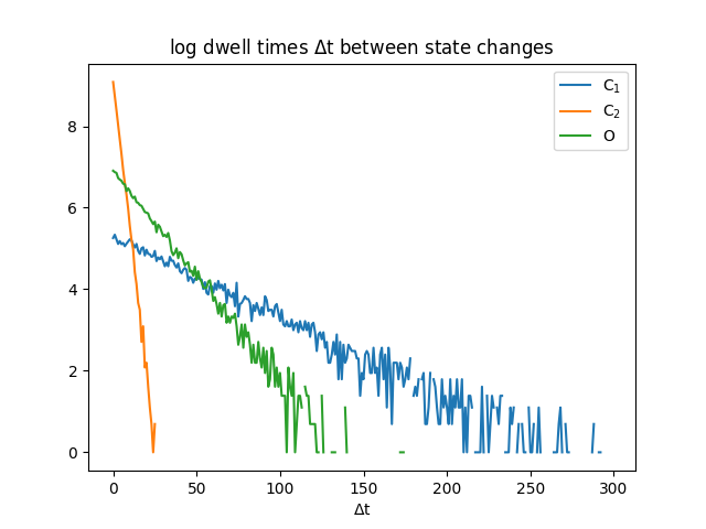
The logarithm of dwell times distribution for each of the 3 states is seen below. We see that state C2 has the shortest dwell times, which makes sense when looking at A_22. Longest dwell times is C1, which makes sense since A_11 is larger than A_22 and A_33. Looking at the distribution between C1 and C2, we can see what would happen, if we didn't know there were 2 states, but thought there was only 1. We will look at the "collapsed" closed states further down.
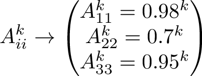
The dwell times are related how long a state will remain in that state, which are given by the diagonal of matrix A. If we are looking at each state being remaining for k time steps, we can see the exponential drop off in probability.
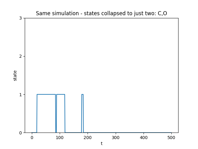
If we intead just measured or observed a single closed state, the simulation would look like below
The dwell time distribution would look like below. We can see that a single exponential distribution does not fit the data very well, which suggests there are more than 1 state
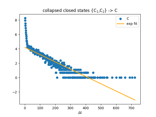
After collapsing the closed states C1,C2 to C, we recounted the dwell times, as would have been done in a real scenario. We then see that the recounted dwell times still have a kink in the distribution, and the linear fit to the log transformed dwell times does not fit the very short dwell time distribution that comes from A_22.
Steady state and eigenvectors
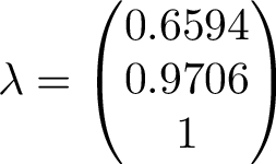
The Markov matrix is a stochastic matrix, so the largest eigenvalue will be 1. This means, over long time, applying the matrix A on an arbritary state vector, the result will converge to the eigenvector corresponding to the largest eigenvalue. The eigenvalues are seen below
The eigenvector corresponding to the largest eigenvalue is the one to the right. We can compare this eigenvector with long term average of our simulation.
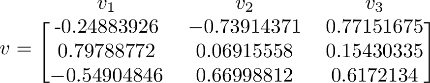
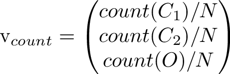
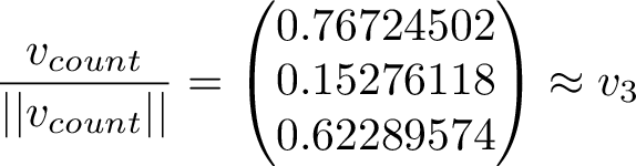
Counting how many times each state occurs and putting the counts in a vector let's us compare the right eigenvector to the long term simulated distribution. The counts from one run gave the values [0.50542, 0.100403, 0.394177].
Scaling the long-term average vector to unit length and comparing it to the 3rd eigenvector, we see they are indeed very close to eachother!
Obviously the count vector will have some random error from the simulation, and also the convergence to the 3rd eigenvector is only as the simulation goes on to infinity.
References
Stephen P. Ellner, John Guckenheimer - Dynamic Models in Biology