Glaciers grow with snowfall, or shrink with ablation. The timesteps here are on the order of years, e.g dt = 1-2 years pr timestep. move few meters pr day at a mostly steady state, hence we can assume acceleration is zero in Newtons second law, and that forces balance eachother out. In particular, surface forces balance body forces.
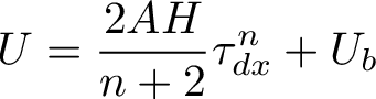
The depth-averaged horizontal velocity is given below. The flow direction is changed when crossing the ice divide. In this model, there is only a horizontal velocity, which is reasonable far away from the ice-divide. Near the ice divide there is significant vertical velocity. That the velocity changes at the divide can also be seen from the velocity, since the slope of the height will shift sign at the divide.
The tau is. This makes sense, the bottom friction increases with H, density and g
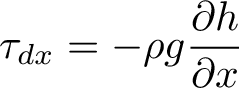
tau also controls the direction of velocity, through the minus sign and the height gradient. If the height increases with x, it makes sense that the velocity of diffusion of ice would go in the opposite direction, to help achieve force balance.
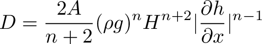
The diffusivity depends on by the gradient of h and H, and the physical values can also depend on location. We thus cannot factor it out in the diffusion equation. For this reason, simulation is a very helpful tool.
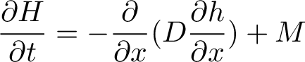
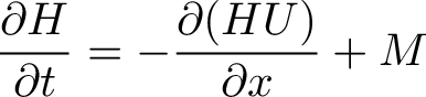
Diffusion equation for ice. Actually the same equation for heat diffusion! In that sense, cold spreads like heat!
Sim. 1 - Linear M
The model here is isothermal and one-dimensional lamellar flow. Drag at the glacier base provides the sole resistance to flow.
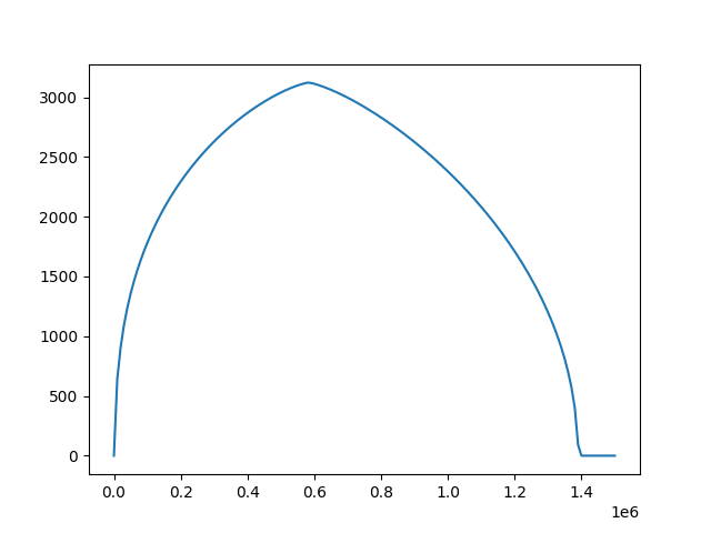
Above is the glacier in the final moments of simulation. It has reached above 3000m in height, and extends further than 1000km.
The full simulation is seen in the animation. We see the ice divide shift southward, and likewise the split for positive and negative velocity direction. For some time, the glacier does not extend beyond the snowfall area at 1000km, but once the glacier grows large enough, the glacier end grows into the next point in the domain, which is a very cool feature of this model and the numerical method.
Sim. 2 - Linear M w/ Lithosphere deflection
Lithosphere (ancient greek Lithos - "rocky") is the outermost rocky layer of planets like Earth. The layer will deflect under the enormous mass of the ice bergs. In 1D, the deflection can be approximated with the same differential equation that is often used in modelling bending of 1D beams. In this case the lithospheric deflection response happens without delay, but in reality the lithosphere will respond to the added weight more slowly
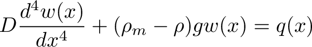
The ODE is 4th order, and hence we need 4 boundary conditions in this 1D case.

The alpha parameter sets the length scale for the problem.
The full animated simulation is shown below
As the glacier grows, the weight will cause larger deflection of the ground.