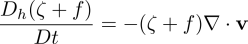
The BVE is a set of equations describing vorticity dynamics, and work reasonable well for oceans and atmospheric processes and the first attempt at prediction the weather using a large computational effort was in the 1950s. The effort was just able to keep up with the actual weather, in that it took just under 12h to do a 12h forecast. To solve the BVE, they had boundary conditions for the streamfunction at all boundary grid points, to solve the Poisson equation. For vorticity, they only needed to specify boundary condition at the inflow points. BVE assumes zero horizontal divergence, which is best fulfilled at around 500hPa, which roughly divides the atmosphere in height by half in terms of pressure. Barotropic fluid assumes that pressure depends only on density. Assuming no frontal zones. The model is limited, but already back then, it was capable of capturing eastward propagation of waves over United States. For synoptic-scale motions, the change of absolute vorticity is related to the divergence by
On a tangential note, the vorticity equations indicates why cyclones(low pressure) can be much more intense than anticyclones(high pressure). For convergence, the relative vorticity will increase in time, while for divergence, it will decrease.
The RHS can be set to zero to achieve conservation of potential vorticity. In essence, far away from surface effects etc, the vorticity will be conserved for columns of air. The resulting equatioms, i.e the barotropic vorticity equation is given by
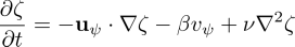
which is the time evolution of the relative vorticity. An eddy diffusion term has been added to RHS. This models the dispersion of energy that comes from eddies of various sizes. Note that is this different from the diffusion that happens at the molecular scale. The simulations are done with channel configuration, which means periodic in x, and bordered in y. The velocity vector is given by the derivative of the streamfunction


At each timestep, we can find the streamfunction by using pseudotime inverse methods for the Poisson equation. The current method works with a simple Jacobi iteration algorithm

The Poisson equation is inversed, with appropiate boundary conditions depending on the scenario. Used BCs are periodic, dirichlet and neumann. Using ghost cells seem to be good at dealing with the various BCs, at least, seems to give less errors. Especially with periodic BCs, you risk losing edge data by just prescribing data from one edge to another edge.
The discretisation is given by Holton, based on the finite difference of the flux form of the PDE.

More advanced methods will discretise the jacobian in different ways, such as the Arakawa method.
Sim. 1 - Double periodic BC
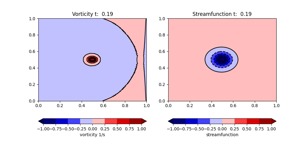
This example is from Chandrasekhar, which contains a solution based on their discretisation. Double periodic. The starting conditions are based below
We use full periodic boundary conditions, with ghost cells the updates for the streamfunction are expressed like below
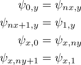
The boundary conditions are applied in every iteration of the Poisson solver. Similar boundary conditions are used for the velocity component and the vorticity.
Chandrasekhar posts a solution for t=0.5, noted below.
Note that although the book uses a different discrete integration method, the solutions are very similar.
Solution is seen below
Sim. 2 Rossby waves - periodic channel
Simulation example, starting with Rossby wave packets. The vorticity, streamfunction and other variables are integrated through time. The Rossby atmospheric waves

Simulations are done for 48h, with a timestep of 100-900s and around 60-200 grid points in each direction. This satisfies Courant conditions.
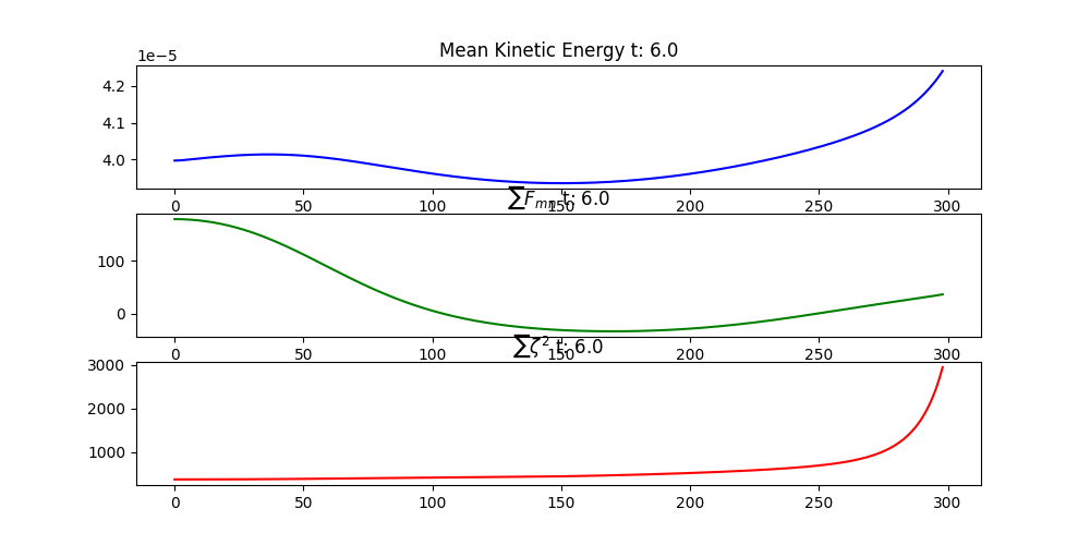
Comparing with initial conditions, we see an eastward propagation of the waves. The initial Rossby wave packets were centered in the domain. The enstrophy and several other quantities are conserved in theory. Some numerical methods achieve this, up to some small oscillations and numerical precision. Arakawa Jacobian is often used for these reasons. The current method uses a flux formulation instead. The enstrophy is given below
Adding orography
We can add mountains of height h to the surface, and add an additional term to the BVE on RHS. This term is discretized again using finite difference method.
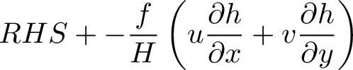
Where H is the average height of the fluid. For 500mb, H is around 5600m. The term depends on the slope of the bottom topograhy, and so steeper mountains will give more abrupt changes in vorticity. Adding these extra terms, can lead to instability, and sometimes the timestep will have to be lowered. Adding e.g two mountains of height 6000
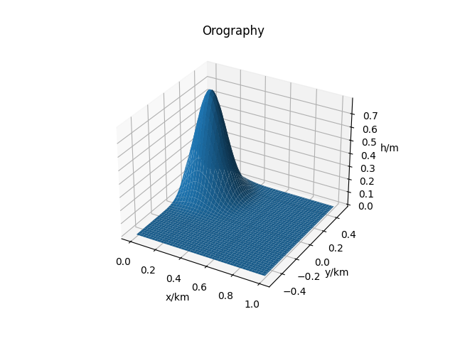
The height from surface texture changes the relative vorticity and streamfunction
Sim. 4 University of Exeter Practical Assignment
Case from university course. https://empslocal.ex.ac.uk/people/staff/dbs202/cat/courses/MTMW14/notes2006.pdf. Boundary conditions are channel, periodic in x, and dirichlet on y. In this case, what I found works best, is updating the north and south streamfunction boundary on each iteration in the Poisson solver. Data are read from msc11.dat, which is found online. These are 500mb geopotential observations, which are converted to streamfunction.
Solution in time is seen below. We see areas of positive vorticity south and negative vorticity north. The negative vorticity areas combine to one, and the positive vorticity area moves north as time goes on.